
Instrumented Systems – SIL Calculations
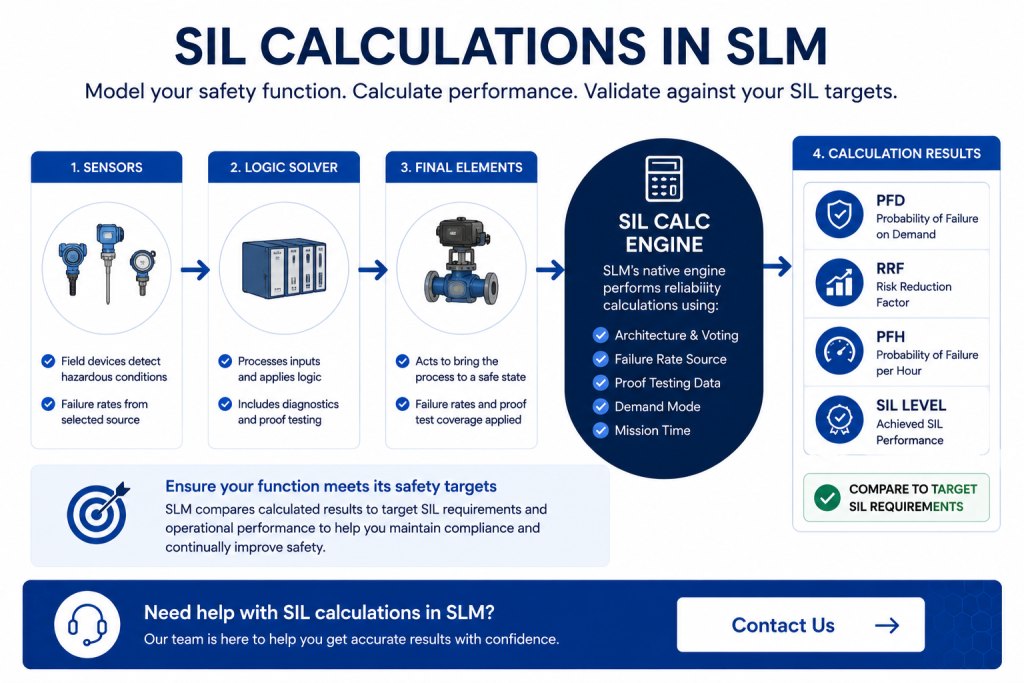
SIL calculations are a critical part of designing, validating, and maintaining Safety Instrumented Functions (SIFs) and High Integrity Pressure Protection Systems (HIPS). Within Safety Lifecycle Manager (SLM), users can perform SIL calculations using the native SIL Calc engine and compare results against target safety requirements and operational performance data.
By combining function architecture, failure rate sources, proof testing information, and demand mode selections, SLM enables organisations to evaluate whether their safety functions achieve the required level of risk reduction. The results can then be compared directly against target SIL requirements and observed operational performance.
This guide explains how SIL calculations work in SLM, the key parameters that influence results, how different failure rate sources are used, and how calculated results are compared against target requirements.
What Are SIL Calculations?
SIL calculations are mathematical evaluations used to determine whether a Safety Instrumented Function can achieve its required Safety Integrity Level (SIL). These calculations typically evaluate the probability of failure on demand (PFD), risk reduction factor (RRF), probability of failure per hour (PFH), and related reliability metrics.
Within SLM, SIL calculations can be executed for both SIF and HIPS functions using the built-in SIL Calc engine.
The calculation process uses:
- Function architecture and voting arrangements
- Failure rate sources
- Proof testing information
- Diagnostic coverage assumptions
- Mission time parameters
- Demand mode selections
The resulting calculations help determine whether the function is capable of achieving the required risk reduction specified during the safety lifecycle.
If you’re new to functional safety terminology, our Safety Integrity Levels (SIL) Explained guide provides an overview of how SIL ratings are determined and applied throughout the safety lifecycle.
How to Calculate SIL Using Function Architecture
One of the most important factors affecting SIL calculations is the architecture of the safety function itself.
Within SLM, users define the sensors, logic solvers, and final elements that make up the function. Voting arrangements determine how many elements must successfully operate for the function to respond to a demand.
SLM uses fault-tree style Boolean algebra calculations to evaluate these configurations.
Voting is expressed as M out of N:
- M = Number of successful elements required
- N = Total available elements
Examples include:
- 1oo1 (1 out of 1)
- 1oo2 (1 out of 2)
- 2oo3 (2 out of 3)
Correct architecture and voting configuration are essential because even small changes can significantly affect the resulting PFD and RRF values.
SIL Calculation Parameters That Affect Results
Accurate SIL calculations depend on the quality and completeness of the input parameters supplied to the calculation engine.
Several fields directly influence calculation outcomes, including:
- Mission Time
- Beta Factor
- Dangerous Failure Percentage
- Proof Test Interval (PTI)
- Proof Test Coverage (PTC)
- Diagnostic Coverage (DC)
- Mean Time To Repair (MTTR)
- Partial Stroke Test Interval (PSTI)
- Partial Stroke Test Coverage (PSTC)
Blank numerical fields are treated as zero values by the SIL Calc engine. As a result, incomplete data can significantly influence calculated results.
SLM also supports automatic unit conversions, allowing users to enter values using different units of measure while maintaining consistent calculations internally.
Probability of Failure on Demand (PFD) Explained
Probability of Failure on Demand (PFD) is one of the most widely used outputs generated by SIL calculations.
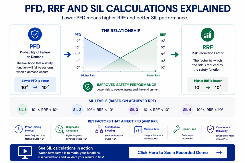
PFD represents the likelihood that a safety function will fail to perform when a demand occurs.
Several factors influence PFD values:
- Failure rates
- Proof testing frequency
- Diagnostic coverage
- Mission time
- Voting architecture
- Repair intervals
Generally:
- More frequent proof testing lowers PFD.
- Higher diagnostic coverage lowers PFD.
- Improved architecture lowers PFD.
- Longer proof test intervals increase PFD.
SLM automatically calculates and displays PFD values based on the selected demand mode and failure rate source.
PFD values play a major role in determining whether a function can achieve its required Safety Integrity Level. Learn more in our SIL 2 Explained and SIL 3 Explained guides.
Risk Reduction Factor (RRF) and SIL Calculations
Risk Reduction Factor (RRF) is closely related to PFD and forms an important part of many SIL calculations.
RRF represents the amount of risk reduction provided by a safety function.
As PFD decreases, RRF increases.
This means that a lower probability of failure results in a greater reduction in risk.
SLM automatically calculates RRF alongside PFD and displays both values within the SIL calculation results.
These values can then be compared directly against target SIL requirements established during design.
Understanding Delete vs Delete and Cascade
SLM provides two distinct deletion options that serve different purposes.
| Option | Purpose |
|---|---|
| Delete | Removes a single eligible object that has no blocking child relationships. |
| Delete and Cascade | Removes an object and all associated descendants within the hierarchy. |
Selecting the correct option helps prevent accidental data loss while ensuring hierarchy structures remain valid.
Users should always review the objects affected before confirming any deletion activity.
Failure Rate Sources Used in SIL Calculations
SLM provides four different failure rate sources for use within SIL calculations.
These sources allow organisations to evaluate results using different assumptions and levels of operational experience.
The available sources are:
- Prior Use Failure Rate – Based on event data captured through Prior Use Certificates.
- Custom Failure Rate – User-entered failure rate values.
- Design Basis Failure Rate – Static values stored within Prior Use Certificates.
- External Results – Results entered from external SIL calculation tools.
Each source may produce different results, and organisations must select which source will govern performance comparisons and reporting.
For organisations managing operational performance data, prior use certificates can provide increasingly accurate results as more event information is collected.
Choosing Between Low Demand and Continuous Demand Modes
The demand mode selected for a function has a significant impact on SIL calculations.
SLM supports both Low Demand Mode and Continuous Demand Mode as defined within IEC 61511.
Low Demand Mode
- Most commonly used mode.
- Results displayed as PFD and RRF.
- MTTFS displayed in years.
Continuous Demand Mode
- Used when demands occur more than once per year.
- Results displayed as PFH.
- SIL levels displayed directly.
- MTTFS displayed in hours.
Changing demand modes does not require users to manually update component parameters because SLM automatically handles unit conversions during recalculation.
Comparing SIL Calculation Results to Requirements
Once SIL calculations have been executed, SLM automatically compares the results against target requirements.
Results are displayed using visual indicators that quickly show compliance status.
- Green indicates the target requirement has been met or exceeded.
- Red indicates the target requirement has not been achieved.
Users must then select a governing result source that determines which calculation result is used for reporting and performance comparisons.
The selected governing source is displayed throughout the function performance views and higher-level reporting structures.
This allows organisations to consistently evaluate safety performance using their chosen calculation methodology.
When reviewing calculation results, it is important to understand the reliability requirements associated with each SIL target. Our guides covering SIL 1, SIL 2, SIL 3, and SIL 4 explain the requirements and risk reduction expectations for each level.
Best Practices for SIL Calculations
Producing reliable SIL calculation results requires more than simply entering data into the system.
Recommended best practices include:
- Verify voting architecture before calculations.
- Ensure proof test intervals are realistic.
- Use accurate diagnostic coverage assumptions.
- Maintain high-quality prior use certificate data.
- Select the correct demand mode.
- Review governing result source selections carefully.
- Validate calculation inputs regularly.
Following these practices helps ensure calculated results accurately reflect real-world safety performance.
For organisations implementing broader functional safety programmes, see our Functional Safety Management Software resources.
Learn More About SIL Calculations and Functional Safety
Understanding SIL calculations is essential for designing, validating, and maintaining effective Safety Instrumented Functions. By combining architecture modelling, failure rate management, proof testing assumptions, and operational performance data, SLM provides a powerful platform for evaluating safety function performance.
You may also find these resources useful:
For additional information on SIL determination and safety lifecycle requirements, visit the International Electrotechnical Commission (IEC).
Instrumented Systems – SIL Calculations
0:06
Welcome to this Application Explainer video, part of our Instrumented Systems topic range.
0:10
In this video, we’ll cover the subject of seal calculations within SLM.
0:16
Within the SLM Instrumented Systems module, users can run seal calculations for SIF and HIPS functions with SLM’s native SEAL Calc engine using various failure rate sources.
0:27
These results can then be compared to the target seal requirements as well as observed failure on demand results tracked in the Operate and Maintain module.
0:35
The following information will be covered in this training.
0:37
Chapter one will be SIF and HIPS function architecture, Chapter 2 will be required calculation parameters, Chapter 3 will be prior certificate usage, Chapter 4 will be failure rate sources, Chapter 5 will be demand modes, and Chapter 6 will be comparison to the requirements.
1:00
In Chapter 1 we will cover your functions, voting architecture, and things to consider, ensuring correct voting at various group levels and keeping instruments part of the function but not contributing to the seal calculation.
1:15
Within the Instrumented Systems module for SIF and HIPS functions, users will generate sealed calculations and results that compared to the target sealed requirements, entered either manually or automatically from the associated local data.
1:30
To execute this calculation accurately as the function is intended to be designed, the functions, architecture and voting must be ensured to be correct.
1:39
The SLM sealed Calculation engine equations utilise fault tree type Boolean algebra calculations that must be voted in terms of how many elements must be successful for the function to activate.
1:52
For instance, in the example displayed, the final element voting requires only one out of the two elements to successfully respond for the function to safely act when experiencing a demand.
2:03
Voting at each layer in the function can be seen in the seal calculation diagram where each element that is filled in with colour represents an element that is contributing to the voting at the next highest level.
2:15
Elements and paths that are not colour field represent elements but do not contribute to the seal calculations.
2:22
In the example presented here, the LT107AB and C sensors will will contribute to the sealed calculations through the path of the high high group, whereas the HS107 hand switch whilst present in the function will not contribute to the calculation due to the manual element not being included in the high group voting.
2:46
If any voting in the functions architecture needs to be modified, tables below the function diagram contain the voting configuration where this can be performed as generic voting is termed M out of North.
3:02
The M field value should be entered as a number of elements that must successfully activate, while the N value is the total number of elements that are available to activate.
3:12
This M number is not entered by the user, but it’s determined by the system from the elements selected in the group.
3:22
In Chapter 2, we will cover data fields requiring entered values for correct or accurate calculation results, and things to consider.
3:30
Blank or empty fields are considered zeros for purposes of the SEAL CALC equation.
3:35
SLM understands unit of measure conversions and will internally convert the unit of measure if the wrong one is selected.
3:42
The number of fields should be entered mostly for the sensors and final elements to ensure an accurate SEAL CALC result.
3:51
It’s important to understand with these parameters that blank value in a numerical field will be treated by SLM seal calculation engine as equivalent to a 0 number value on each voting element.
4:02
A beta factor is available to specify, although it’s not always required.
4:08
The beta factor is the percentage of the failure rate of the voting group attributed to single faults that lead to the failure of multiple components.
4:19
Lower assumed beta values will yield lower probability of failure on demand or PFDS and higher RRFS.
4:27
When the M value of a voting configuration that is an M out of N is equal to N, then the beta factor will become irrelevant and there then will reset any entered value to 0.
4:39
For example, if I change this value on a beta value on a one out of one voting configuration to 5% and then click on save, the system will reset the beta value to zero.
4:55
However, if my M value does not equal my N value such as this 2 out of 3 voting and I changed my beta to 5%, the system will save that value as entered.
5:09
Mission time is the period of time when the SIF or device is put into service and when it is replaced or completely refurbished to an as new condition.
5:19
This interval essentially resets the accumulated uncovered failures TO0A.
5:24
Shorter interval is associated with higher still results, but typical mission time intervals fall somewhere between 15 and 30 years.
5:33
The remaining parameter fields are entered on the individual input, logic, solver, and output components and are not contextual to each parent function.
5:42
Meaning, if two functions use the same sensor or final element, changing a parameter of the component under one function will result in the same parameter being changed under the second function.
5:53
When this occurs, SLM will flag function 2 as having a pending steel calculation that must be confirmed by the user to execute.
6:02
Dangerous failure percentage All failure rates are assumed to be a total failure rate incorporating both dangerous and safe failures.
6:11
The danger failure percentage field is applied to the custom failure source.
6:15
If the custom failure rate is assumed to be the only dangerous failures, enter a value here of 100% custom failure rate.
6:24
In order to experiment with different failure rates or if a suitable prior use certificate option is not available, the failure rate values could be entered manually for each component.
6:35
Proof Test Interval Proof Test interval or PTI is the period interval time between testing of the component.
6:42
The PTI value may be entered in the unit of measure of your choice for each component as SLM will internally translate the unit of measure to be consistent with other components.
6:59
Longer time periods here will yield higher PFDS or lower RRFS for the SIF proof test coverage.
7:08
A proof test is not likely to detect all failures before their potential occurrence.
7:13
The proof test coverage is an assumed percentage of the failures based on the proof testing procedures that are expected to be discovered during a proof test.
7:22
A higher PTC percentage will load lower PFDS or higher RRFS.
7:28
For the SIFT diagnostic coverage.
7:32
The diagnostic coverage, or DC is the ratio of the probability of detected failures to the probability of all detected and undetected failures.
7:42
Diagnostic tests are employed to decrease the probability of dangerous hardware failures.
7:48
Being able to detect all dangerous hardware failures would be ideal, but in practice the maximum value is set to 99%.
7:55
Higher assumed DC percentages will yield lower PFDS or higher RRFS.
8:01
For the SIF, this value is always entered in percent Meantime to repair.
8:08
The Meantime to repair or MTTR is the time required to repair the component after a failure is detected.
8:16
Because a failure must be detected in order to repair it before the demand were to occur, the MTTR parameter only affects the detected failure’s portion of the calculation.
8:26
While this is normally a negligible contributor to the calculation result, longer MTTR periods are associated with higher PFD results.
8:36
This value is always entered in terms of hours on the output or final element object.
8:43
Two more parameters are associated.
8:48
The partial stroke test interval improves the overall SIFT reliability by uncovering the faults through partial movement of the final elements.
8:58
The PSTI value is entered in units of months and more often testing or shorter intervals will yield lower PFDS and higher RRFS.
9:07
The partial stroke test coverage, or PSTC is the percentage of the failures that are discovered through partial stroke testing at the final elements.
9:17
Higher assumed percentages will yield lower PFDS or higher RRFS.
9:21
Although realistic coverage is no more than around 60%, this value is always entered in percent.
9:30
In Chapter 3, we’ll cover selecting instrument prior use certificates and things to consider.
9:36
PU CS are assigned to the instrument tag itself, which may be shared with other functions.
9:42
APUC may not yet have enough recorded events to reflect an accurate prior use Silk ALC result.
9:49
Prior use certificate usage for any sensor or input logic solver or final elements or output.
9:58
Prior use certificates may be available to select and apply to a particular components.
10:04
The list of these prior use certificates or Pucs that are available for use are managed in the global or Operate Maintain module.
10:12
Selecting Pucs for components here would directly affect the sealed CAC results for the prior use and the design basis failure rate sources in the prior use certificate data.
10:24
The design basis failure rate is directly entered and stored as a static value for use by the sealed calculations when the PUC is selected for the components.
10:33
Additionally, as event data such as demands, tests, bypasses, etcetera is captured and recorded within SLM for the devices associated with particular prior use certificates, the prior use failure rate for the PUC will be updated by SLM dynamically, giving a more accurate failure rate and seal calculation based on the experience performance of the device type in the inputs table of the Seal Calc architecture of the SIF, the prior use certificate for each input object may be selected by first selecting the input function, the process measurement, then the input type fields.
11:11
These field selections will drive the available prior use certificates to select from.
11:16
In the Logic Solvers table, the Logic Solver function, the Logic solver type, and the Logic solver Manufacturer field must be selected before selecting a PUC, and similarly, in the Outputs table, only the Output function and the Output type fields must be selected before choosing a PUC.
11:44
With the PUC selected for these components, SLM may then provide a sealed calculation result for the prior use and design basis.
11:52
Failure rate sources.
11:56
In Chapter 4, we’ll cover which failure rate source to select in governing results, things to consider, accuracy of various failure rate sources, and mean time to failure versus risk reduction factor results.
12:10
Failure rate sources with the function sealed calculation executed and complete SLM will provide four different results based on four different failure rate sources.
12:20
Source one is the prior use failure rate source and is determined from the prior use certificate selections made within each component.
12:28
As mentioned in the previous chapter, the resulting PFD RRF calculation is dynamically affected by the device events that captured and stored in SLM’s Operate and Maintain module.
12:39
Note that the accuracy of sources will be dependent on the amounts and completeness of the device event data that is captured in SLM.
12:47
The second source is the custom failure rate source and is calculated from the Custom failure rate field on each input logic solver and Output component.
12:57
This is useful in the case that no prior use certificates are selected and a sealed calculation result is still desired, so SLM may still calculate APFDRRF result to compare with the target requirements.
13:09
The third source, the design basis failure rate, is determined in parallel for the prior U source by ensuring that PUC selections are made for each component.
13:19
The difference between these two sources being that the design basis failure rate result is based on a static value entered within the PUC and therefore will not dynamically change with the event data captured.
13:30
The final or full failure rate source is the external result, and this source is exactly what it seems to be, a sealed calculation result From an external calculation source, each PFD group value may be entered manually, which will then be summed into the total PFD and inverted for the total RRF value.
13:52
It’s important to note that the external result values are expected to be entered in units of per year when the function is in low demand mode, but units of per hour when the function is in continuous demand mode.
14:04
Another item of note in this table is the MTTFS or Meantime to fail spurious.
14:10
This value will be calculated for each source alongside the total PFD RF value for each failure rate source, with the exception to the external result source, which also must be entered manually.
14:22
The MTTFS value is affected by many of the same parameters affecting the sealed calculation result covered in Chapter 2 and gives an indication of the trip sensitivity of the function.
14:33
For example, if the total RF is calculated to exceed the target requirements, but the MTTFS value is lower, then the function can be thought to be reliable but bring the process to a safe state.
14:45
In an emergency, however, a large number of unwanted process upsets should also be expected.
14:51
Having both values displayed in this table can help with both the design architecture or voting configuration at the functions as well as the selected failure rate source.
15:05
In Chapter 5, we’ll cover choosing the correct demand mode the actual function is experiencing and things to consider.
15:13
What is the expected rate of demand on the function and which demand mode to assume is determined by the IEC 61511 regulations?
15:23
SLM silt calc engine is capable of providing results in either of two modes of operation.
15:29
These modes of operation are selected in the demand mode field and correspond with the SIFT modes of operation as defined in IEC 61511, Part 1.
15:40
When the low demand option is selected for the function in SLM, the Cilk AC result will be calculated and displayed in terms of probability of failure on demand and risk reduction factor, with meantime to failure spurious in units of years.
15:55
This mode of operation is the most common and most likely to be selected for each function.
16:00
When a function’s expected frequency of demand is greater than once per year, or if the function retains a process in a safe state, the demand mode should be set to a continuous demand mode and SLM will calculate and display results accordingly.
16:15
SLM will display the results in terms of failures per hour and the corresponding safety integrity level, with the mean time to failure spurious now in units of hours.
16:26
When changing the functions demand mode, it’s not necessary to modify any of the functions component parameter fields as SLM is capable of internally converting the units of measure appropriately.
16:37
The only required action to be taken upon changing the demand field selection is to execute the command to update seal calculations.
16:46
This will trigger SLM to recalculate the seal calculations in the appropriate PFD or PFH results in units.
16:58
In Chapter 6, we will cover comparing the seal calc result to the required reliability target of the function and things to consider which failure rate source is used in governing result source and if a safety factor padding above the target is required.
17:14
With SLM having produced sealed calculation results, a comparison to the target requirements will be displayed automatically in the function sealed calc result table.
17:25
Any result that is highlighted in green is meeting or exceeding the target requirement, while any result in red is less than or not meeting the target requirements.
17:34
At this point, it is necessary to choose which failure rate source will be the governing result for the function, which can be selected in the governing results source field.
17:42
On selecting an option SLM, use the result value corresponding to the selection in the comparison fields and tables.
17:49
In the performance view of the function, the result of the selected governing source will be displayed in a table with a direct comparison to the target requirements and in the unit a high level organization levels.
18:01
In the sealed Calc OPS view, the function will be reported in the appropriate comparison table, either failing or meeting the function’s target requirements.


